How to Freeze a Row in Google Sheets (Desktop + Mobile)
Freeze rows and columns in Google Sheets in seconds. Step-by-step guide for desktop and mobile, plus fixes for the most common freezing issues.
Quick AnswerTo freeze a row in Google Sheets, go to View > Freeze > 1 row. For multiple rows, click a cell in the last row you want frozen, then choose View > Freeze > Up to current row. On mobile, tap and hold the row number, then select Freeze.
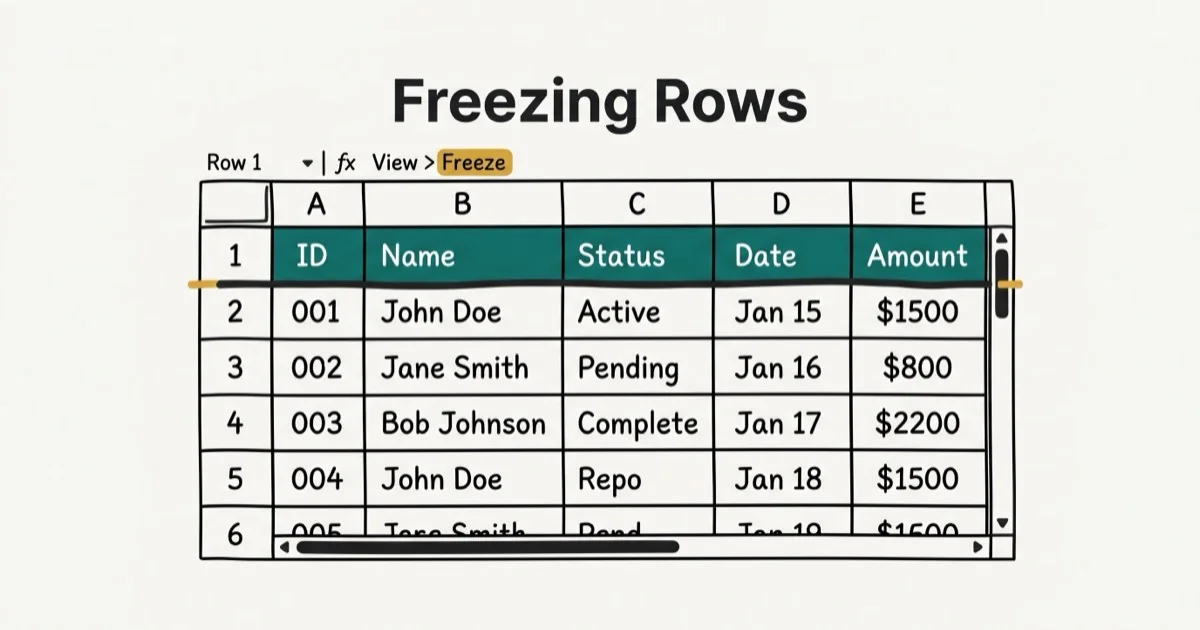
Freezing rows keeps your header visible while you scroll through a long sheet. The View > Freeze menu is the direct way to pin a header row.
- Go to
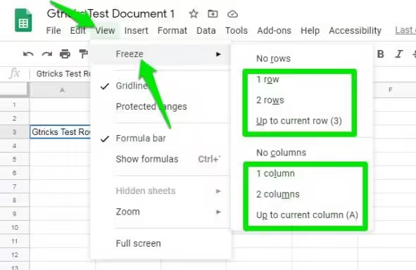
View>Freeze> 1 row to freeze the top row on desktop in one click. - On Android and iOS, tap and hold the row number, then select Freeze from the menu.
- You can freeze up to 10 rows, but they must start from the top of the sheet.
- Combine row and column freezing via
View>Freeze> 1 column for both axes at once. - To unfreeze, go to
View>Freeze>Norows, or drag the freeze bar back to the top.
#Freeze the Top Row on Desktop
Open Google Sheets in your browser. Go to View > Freeze > 1 row. A thick gray line appears below row 1. Scroll down and the header stays put.
The View menu method applies the freeze as soon as you select it. Start here for the fastest result.
#Freeze Multiple Rows on Desktop
For multiple rows:
- Click any cell in the last row you want frozen. Click a cell in row 3 to freeze rows 1 through 3.
- Go to
View>Freeze>Upto current row. - A thick gray bar under the frozen section confirms it worked.
You can also use the drag handle. Hover over the small gray square in the top-left corner where row and column headers meet. Drag it down to set the freeze point.
The View menu method is more precise when you need an exact row number. The drag handle is faster when your mouse is already at the corner.
#Freezing Rows on Mobile Devices
The process differs slightly between Android and iOS.
On Android: Open Google Sheets. Tap and hold the row number on the left side. Tap Freeze in the context menu.
On iOS: Tap the row header number. Tap the blue arrow that appears. Then tap Freeze.
The frozen row shows a slightly darker border on mobile to confirm the freeze is active.
#Can You Freeze Both Rows and Columns at Once?
You can freeze both rows and columns and both stay pinned simultaneously.
- Freeze rows first:
View>Freeze> 1 row. - Then freeze columns:
View>Freeze> 1 column.
Google’s official Sheets documentation states that you can freeze up to 10 rows simultaneously. You can also freeze up to 5 columns at the same time. Both stay pinned when you scroll in any direction, and the limit applies to free Google accounts, not just Workspace plans.
This setup is useful when you need both a row header and a key column visible. The freeze setting syncs across collaborators.
#Why Are Your Frozen Rows Not Staying Fixed?
Rows won’t stay frozen after refresh. Clear your Chrome cache and re-apply the freeze. If it keeps happening, try a different browser profile after clearing cache.
Frozen rows don’t print. In the print dialog, go to Headers and Footers and check “Repeat frozen rows.” According to Google’s guide to freezing rows and columns, frozen rows appear in exported .xlsx files automatically, but repeating them on each printed page requires enabling this specific checkbox under File > Print > Headers and footers.
Can’t select the rows you want. Click the row number on the far left edge, not a cell inside the row. Then choose View > Freeze > Up to row N.
#How to Unfreeze Rows in Google Sheets
Two ways to remove a freeze:
- Menu method: Go to
View>Freeze>Norows. All frozen rows release instantly. - Drag method: Hover over the thick gray freeze line until you see a hand cursor. Drag it back up to the top-left corner.
Google’s help center confirms that unfreezing via menu resets all frozen rows at once. You can’t unfreeze individual rows without clearing the whole freeze. If you only want fewer rows frozen, clear all first and re-apply the freeze to the new row number.
#Bottom Line
Use View > Freeze > 1 row. That covers 90% of use cases. If you need both row and column headers locked, freeze them separately from the same View menu.
For shared spreadsheets, combine frozen rows with locked cells in Google Sheets to prevent accidental edits. You can also highlight duplicates in Google Sheets while your header stays visible.
For managing headers in text documents, see how to delete headers in Google Docs. If you work in Excel too, check how to unprotect an Excel sheet without a password when you inherit a protected workbook.
Imported sheets with external dependencies sometimes need cleanup too. Learn how to break links in Excel before sharing the file with collaborators.
#Frequently Asked Questions
How many rows can you freeze in Google Sheets?
You can freeze up to 10 rows. They must start from row 1 and be contiguous. You can’t freeze row 5 without also freezing rows 1 through 4.
Does freezing rows affect formulas or data?
No. Freezing is purely a visual display setting. Your formulas, cell references, and values stay exactly the same. Nothing in the underlying spreadsheet data changes.
Can you freeze rows in the middle of a spreadsheet?
No. Google Sheets only supports freezing rows from the top of the sheet. If you need a row in the middle visible, duplicate it as a header in row 1 and freeze that row instead.
Why did frozen rows disappear on a shared spreadsheet?
Another collaborator likely unfrozen them. Freezing is a per-file setting shared by all editors, not a per-user view.
To prevent it happening again, go to Data > Protect sheets and ranges and restrict who can edit the header row. That way the freeze setting and the header content stay intact. Reapply the freeze after setting up protection.
Do frozen rows show up when you download the spreadsheet?
Yes. Downloading as .xlsx transfers the freeze setting to Excel. CSV format has no visual formatting, so the freeze doesn’t apply there, but row order stays intact.
Can you freeze rows in the Google Sheets mobile app?
Yes, on both Android and iOS. Tap and hold the row number, then tap Freeze. The mobile app supports up to 10 frozen rows, the same limit as desktop.
What is the difference between freezing and locking rows?
Freezing keeps rows visible while scrolling. Locking (protecting) prevents editing those rows. They work independently and you can apply both at the same time for full control over header rows.
Apps Crashing After iOS 27 Update? Fix Order (2026)
Apps crashing after the iOS 27 update? Update the app in the App Store first, then offload and reinstall to clear stale cache, then restart. The fix order.

Do AI Translation Earbuds Work Offline? What to Know
Do AI translation earbuds work offline? A few do with downloaded language packs, but most need the cloud. Here's what works offline and what you give up.

How to Set Up Translation Earbuds (Pairing and Modes)
How to set up translation earbuds: charge, install the app, pair over Bluetooth, pick two languages, and choose a mode. A step-by-step first-use guide.

Translation Earbuds Not Translating? How to Fix Them
Translation earbuds not translating? Usually it's the app, the internet, or the language settings. Here's how to fix pairing, sound, and lag fast.