How to Highlight Duplicates in Google Sheets (2026)
Highlight duplicates in Google Sheets with one COUNTIF conditional formatting rule. Step-by-step guide for single columns, multiple columns, and rows.

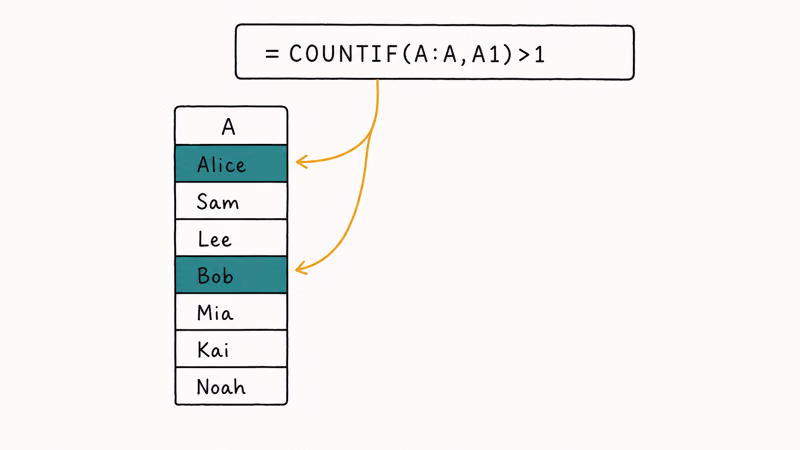
Quick AnswerSelect your data, open Format > Conditional formatting, choose Custom formula is, enter =COUNTIF(A:A, A1)>1, pick a fill color, and click Done. Sheets paints every cell whose value appears more than once in the column.
Highlight duplicates in Google Sheets with one conditional formatting rule and a single COUNTIF formula. No add-on, no script needed. The pattern works for a single column, a multi-column block, or entire rows, and it updates the moment you edit a cell.
- The base rule is
=COUNTIF($A:$A, $A1)>1insideFormat>Conditional formatting > Custom formula is. Replace the column letter and click Done. - Conditional formatting is live: when you edit, paste, or import a new row, Sheets recolors duplicates without a refresh.
- For multiple columns, select the block and use
=COUNTIF($A$2:$D, A2)>1. Anchor the search range with dollar signs, leave the test cell un-anchored. - To color whole rows, set the Apply to range to the full data block (for example A2) and use
=COUNTIF($A$2:$A, $A2)>1so every cell in that row inherits the fill. - Flip the comparator to
=COUNTIF($A:$A, $A1)=1and you get unique values highlighted instead, which is handy for finding one-off entries in a long list.
#What Counts as a Duplicate in Google Sheets?
A duplicate is any value that appears more than once inside the range you tell Sheets to check. That sounds obvious until you remember that John Smith and john smith (trailing space) are different to a spreadsheet but look identical to a human. Conditional formatting only sees the raw value, not the visible text.
That gap shows up in three common places:
- Customer lists where the same person was entered as
Mary O'Neil,mary oneil, andMary O'Neil(the last one carries a hidden space). - Imported transaction logs that look duplicated to the eye but carry invisible non-breaking spaces or different currency symbols.
- Inventory exports with SKUs that round-trip through Excel and pick up apostrophes or stored-as-text formatting.
The fix is to clean before you highlight. Wrap the value in TRIM() and LOWER() inside the COUNTIF formula, or run Data > Data cleanup > Trim whitespace once before applying the rule. Skip this step and you’ll color half your real duplicates and miss the rest.
#Highlight Duplicates in a Single Column
This is the workhorse case. One column of values, anything repeated gets a fill color. The steps are short.
- Click the column header (or drag to select the data range, for example A2).
- Open
Format>Conditional formatting from the top menu. - Under “Format cells if…”, pick Custom formula is.
- Enter
=COUNTIF($A:$A, $A1)>1. Match the column letter to the column you selected. - Pick a fill color under “Formatting style”. Yellow is the conventional choice.
- Click Done.
Two parts of the formula matter. The $A:$A is the search range with absolute references so it stays locked across every row. The $A1 is the current cell, with only the column locked.
The row reference floats so the rule walks down every row in your selection. Swap those and the rule either paints nothing or paints everything.
According to Google’s conditional formatting documentation, custom formula rules accept exactly 1 formula per condition and evaluate against the top-left cell of the applied range, which is why the row reference must remain unanchored. The rule is also live. Paste a new row, and Sheets recolors duplicates without re-running anything.
Conditional formatting usually stays responsive on modest ranges. If the applied range gets very large or very wide, Sheets can slow while scrolling or editing.
#How Do You Highlight Duplicates Across Multiple Columns?
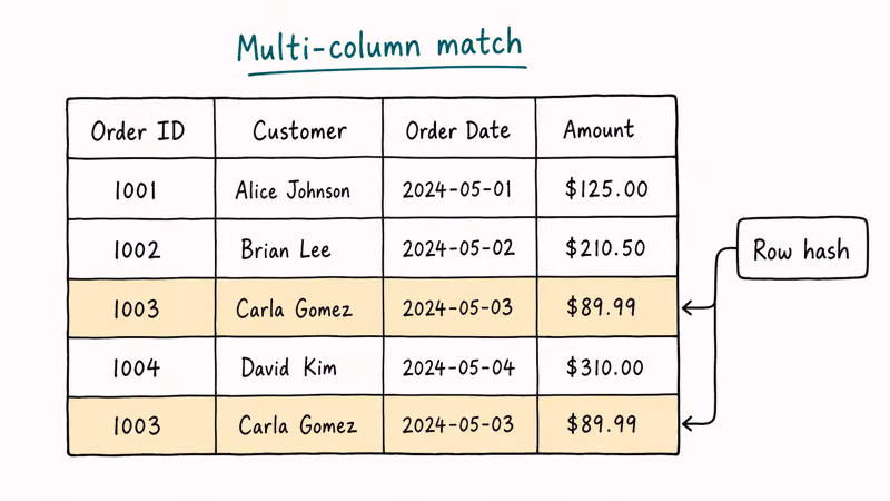
For a wide table where any repeat across all columns should be flagged, you point COUNTIF at the entire block instead of a single column.
- Select the full data block, for example A2.
- Open
Format>Conditional formatting. - Choose Custom formula is.
- Enter
=COUNTIF($A$2:$D, A2)>1. The first argument is the locked block; the second argument is the current cell with no dollar signs so it walks. - Pick a color and click Done.
Note the trailing range. $D without a row number means “to the bottom of the data.” That’s deliberate. Set a hard upper bound like $D$500 and a 501st row escapes the check.
Google’s COUNTIF function reference states that COUNTIF takes exactly 2 arguments, a range and a single criterion, which is why the formula scales to whatever rectangle you give it. If you instead want duplicates within each column but not across columns, run a separate single-column rule per column. There is no built-in per-column toggle.
#Highlight Entire Rows That Contain Duplicates
The single-column rule colors only the duplicate cell. If you want the whole row highlighted because, say, the email address repeats, change two things:
- Set the Apply to range to the entire row block (A2, not just column B).
- Use
=COUNTIF($B$2:$B, $B2)>1where column B is the key, the column you’re checking for repeats.
The $B2 reference has the column locked and the row floating, so every cell in row 2 (A2, B2, C2, D2…) evaluates the same key cell and gets the same fill. Want to key off two columns combined? Concatenate them: =COUNTIF(ARRAYFORMULA($B$2:$B&$C$2:$C), $B2&$C2)>1. The ARRAYFORMULA stitches the two columns into a virtual key column at evaluation time.
This is the most useful rule for cleaning subscriber exports. The email column is the key, but you want the whole row colored so it’s obvious what’s getting purged.
#Color-Code Duplicates by Frequency or Type
A single yellow fill is fine for binary “is this a repeat?” work. For dirtier data, layer rules so the color tells you how duplicated something is.
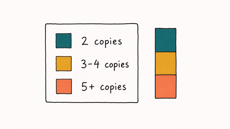
Add three rules in this order. Sheets evaluates top-down and stops at the first match.
- Triple or higher with formula
=COUNTIF($A:$A, $A1)>=3and a red fill. - Exact double with formula
=COUNTIF($A:$A, $A1)=2and an orange fill. - Unique with formula
=COUNTIF($A:$A, $A1)=1and a light green fill.
A glance at the column now tells you which entries need urgent dedup work versus which are just stragglers. The same layering trick works for matched pairs against a reference list. Rule 1 paints “in both sheets,” rule 2 paints “only in this sheet,” rule 3 paints “only in the other sheet.”
For tables where the underlying data needs to stay protected after color-coding, pair this with locking cells in Google Sheets so a teammate can’t overwrite a row you’ve flagged for review.
#Troubleshooting When the Rule Misses Duplicates
When the rule looks right but no fill appears, walk through these in order.
- The range and the formula disagree. If you applied the rule to A2 but the formula starts with
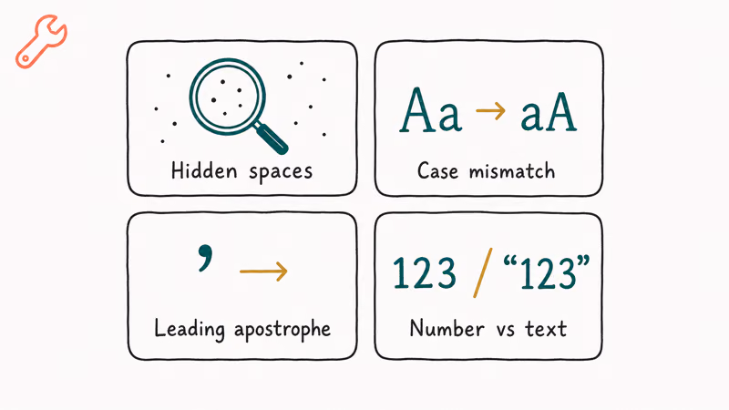
$A$1, the relative offset is one row off. Either start the rule at A1 or change the formula to$A2. - Hidden whitespace.
Run Data>Datacleanup > Trim whitespace, then re-check. Trailing spaces are the most common silent killer. - Numbers stored as text. A SKU column that came in from a CSV may have one row formatted as text and another as a number, and COUNTIF treats
12345and"12345"as different values. Select the column and applyFormat>Number>Plaintext (or Number, consistently). - Multiple rules competing. Sheets evaluates rules top-down. If a “unique” rule sits above your duplicate rule with a broader match, it can win first. Reorder rules so the most specific rule sits at the top.
- The applied range is too wide. Performance also degrades on very wide applied ranges. If your sheet has hundreds of thousands of cells under one rule, the page will drag. Narrow the Apply to range to the actual data block.
If the sheet is sluggish even after a clean rule setup, the bottleneck is usually the dataset size, not the formula. Similar wait patterns appear when Excel stops responding on heavy workbooks, and the diagnostic flow there is parallel.
#Better Alternatives: UNIQUE, Remove Duplicates, and Add-ons
A color rule tells you where the duplicates are. Sometimes you want them gone or summarized instead. Three native options handle that without coloring anything:
- Remove duplicates under
Data>Datacleanup is Sheets’ built-in destructive dedup tool. It keeps the first occurrence and deletes the rest. Always run it on a copy of the sheet first. The action is undoable inside the current session but is hard to reverse after the tab is closed. - UNIQUE function. Type
=UNIQUE(A2:A)into an empty column and Sheets returns a deduped list of values without touching the source list. Add a sort with=SORT(UNIQUE(A2:A))if you want a tidy reference list to share. - Frequency summary. Drop
=QUERY(A:A, "select A, count(A) where A is not null group by A having count(A) > 1 order by count(A) desc")into an empty cell and you get a frequency table of every duplicate, sorted by how often each one repeats.
Google’s Sheets function list confirms that COUNTIFS handles 2 or more criteria simultaneously, which is the function to reach for when one COUNTIF rule isn’t enough. For everything else, COUNTIF plus UNIQUE covers the productivity cases that come up day to day.
Add-ons exist (Remove Duplicates by Ablebits is the popular one), but Sheets’ native tools cover most routine cleanup cases. Add-ons are mainly useful for fuzzy matching across thousands of rows, which is the one job native COUNTIF can’t fake.
#Keep Your Sheet Reliable After the Cleanup
A clean rule helps once. The bigger win is preventing duplicates from accumulating in the first place. Two habits do most of the work.
The first is data validation on entry columns. Set Data > Data validation > Reject input with =COUNTIF(A:A, A1)=0 and a duplicate can’t be typed in at all.
The second is freezing the header row and key column. When you are scrolling a long sheet to spot which highlight color means what, the headers vanishing makes the audit useless. Pin them in place, and our walkthrough on freezing a row in Google Sheets covers the menu path.
When the analysis jumps to Excel (Sheets for live entry, Excel for offline reporting), the trend analysis in Excel guide pairs well with the dedup work here. Lost a cleanup session to a crash? Our walkthrough on how to recover an unsaved Excel file lists the recovery folder paths to bookmark before it happens again.
#Bottom Line
Use one custom-formula conditional formatting rule with COUNTIF as your default. The single-column form =COUNTIF($A:$A, $A1)>1 covers most jobs in under a minute, and the same pattern stretches to multi-column tables, whole-row coloring, and tiered color codes by frequency. Add Data > Data cleanup > Trim whitespace before you apply the rule, and reach for Remove duplicates or UNIQUE only when you want the duplicates gone instead of flagged.
#Frequently Asked Questions
Can I highlight duplicates based on partial matches?
Yes. Use wildcards inside the COUNTIF criterion: =COUNTIF($A:$A, "*"&$A1&"*")>1 matches any cell that contains the current value anywhere in its text. Be careful with short tokens, because “an” will match every cell that contains “an” as a substring.
How do I remove the highlighted duplicates after I’ve found them?
Run Data > Data cleanup > Remove duplicates on the same range. Sheets keeps the first occurrence and deletes the rest, then the color rule recalculates automatically and the remaining cells lose their fill. Always run it on a copy of the sheet first because the action is hard to reverse after the tab is closed.
Will conditional formatting change the underlying data?
No. The rule only paints cells. Values, formulas, and references stay untouched, so it’s safe to apply on a live sheet.
Can I highlight unique values instead of duplicates?
Yes. Change the comparator from >1 to =1: =COUNTIF($A:$A, $A1)=1 paints every value that appears exactly once. That’s the cleanest way to surface one-off entries in a long list.
Is there a row limit for conditional formatting?
There isn’t a hard row limit, but performance drops on very wide applied ranges. Narrow the Apply to range to the actual data block, or split the rule across smaller chunks if your sheet feels sluggish.
Does this work in the Google Sheets mobile app?
Rules created on the desktop web render correctly on the mobile app. The custom-formula editor isn’t exposed in the mobile UI as of 2026, so set the rule on a laptop and the phone will inherit it.
Why are some duplicates in my email column not getting highlighted?
Mixed case combined with trailing whitespace is the usual cause. User@email.com and user@email.com are three different values to COUNTIF. Wrap the comparison with LOWER(TRIM(…)) in both arguments, or run Data > Data cleanup > Trim whitespace first. Then change the formula to =COUNTIF(ARRAYFORMULA(LOWER($A:$A)), LOWER($A1))>1 so the rule normalizes case during evaluation.