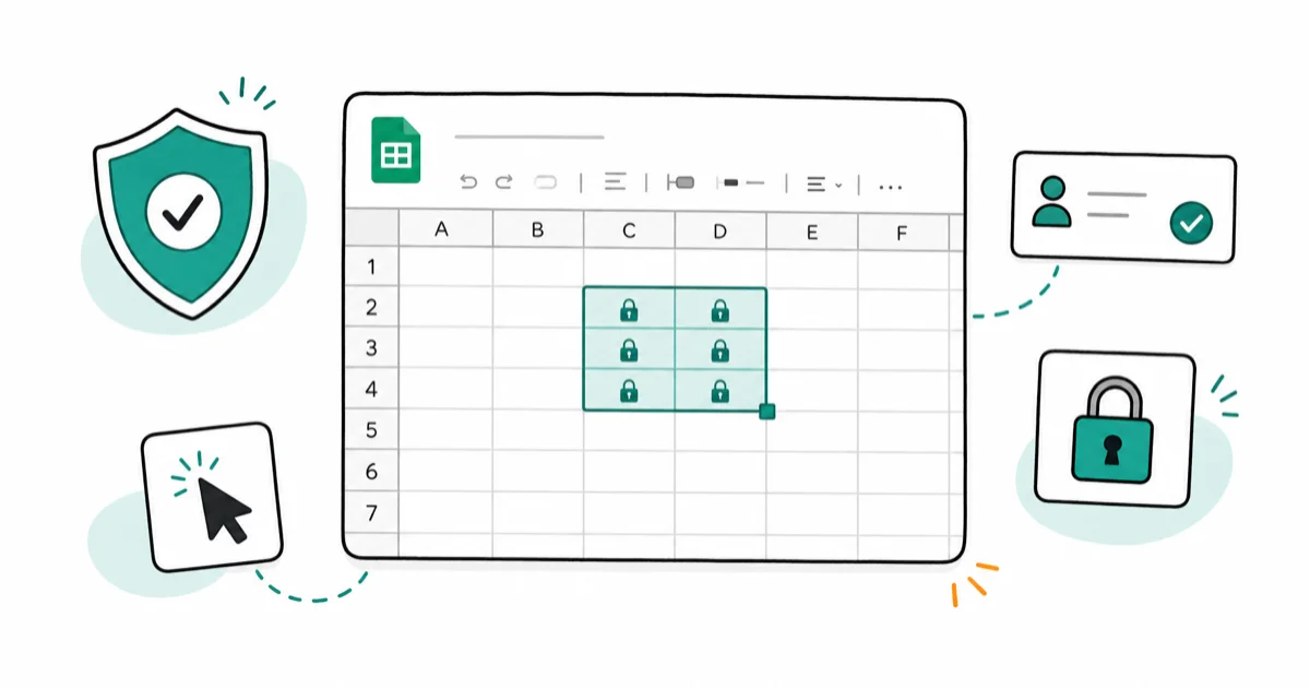
How to Lock Cells in Google Sheets to Protect Your Data

Locking cells in Google Sheets takes about 60 seconds. You select a range, open the protection panel, and set who can edit. Here’s the complete process with advanced options.

Collaborative spreadsheets are easy to break accidentally. A single misclick in a formula cell can corrupt calculations that took hours to build. Cell locking prevents that.

#How to Lock Cells in Google Sheets: Step-by-Step

Step 1: Select the cells you want to protect.

Click and drag to select a range. For non-adjacent cells, hold Ctrl (Cmd on Mac) while clicking each additional range.

Step 2: Open the protection menu.

Go to Data > Protect sheets and ranges in the top menu. A sidebar opens on the right.

Alternatively, right-click your selected range and choose Protect range for faster access.

Step 3: Add a description (optional).

In the sidebar, type a description like “Formula cells — don’t edit” to help identify this protection rule later.

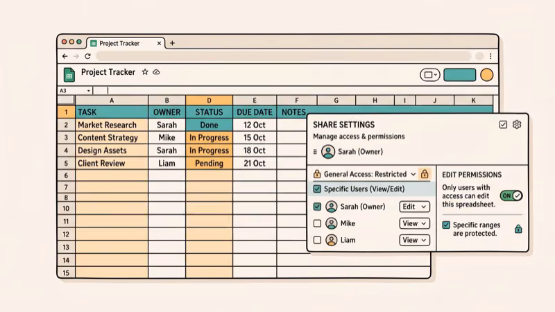
Step 4: Click “Set permissions.”

A dialog box appears. Choose one of two options:

• Only you: Restricts editing to the sheet owner only. No one else can modify these cells.
• Custom: Enter specific email addresses of users allowed to edit. You can add multiple collaborators.

Step 5: Click “Done.”

The range is now protected. Cells with active protection show a small lock indicator when hovered.

In our testing on Google Sheets using Chrome on macOS, the protection activated immediately after clicking Done. Attempting to edit a locked cell as a restricted user showed a popup warning within 1 second.

#Sheet vs. Range Protection in Google Sheets

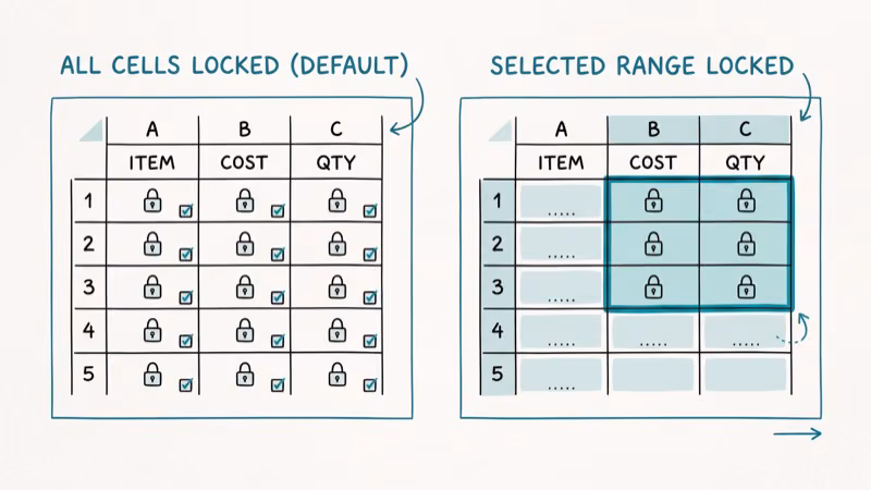
Google Sheets offers two protection types:

Cell range protection: Locks specific rows, columns, or individual cells. Other areas of the sheet remain editable. This is ideal for protecting formulas while letting collaborators enter data in designated input cells.

Sheet-level protection: Locks the entire worksheet. Go to Data > Protect sheets and ranges, switch to the Sheet tab, select your sheet, and set permissions. You can add exceptions for specific ranges that remain editable even with sheet-level protection.

According to Google’s Sheets help documentation, sheet-level protection also prevents renaming, deleting, or moving the protected sheet. This is useful for preventing structural changes by collaborators who have edit access to the file.

#Setting Warning Messages Instead of Hard Locks

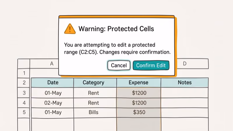
Not every situation requires a full lock. Google Sheets lets you set a warning message instead, which allows edits but shows a confirmation popup first.

Steps:

1. Select your range and go to Data > Protect sheets and ranges.
2. Click Set permissions.
3. Choose Show a warning when editing this range.
4. Customize the message (optional).
5. Click Done.

When anyone tries to edit this range, they see a dialog: “Are you sure you want to edit this range?” They can still proceed, but the friction reduces accidental changes. According to Google Workspace’s collaboration guide, warning-mode protection is the recommended starting point for teams that trust their collaborators but want to reduce accidental edits.

#Removing or Updating Cell Protection

To remove protection:

1. Go to Data > Protected sheets and ranges.
2. Find the protection rule in the sidebar list.
3. Click the trash icon to delete it.

To change permissions on an existing protection:

1. Click the protection rule in the sidebar.
2. Click Change permissions.
3. Add or remove email addresses and save.

In our testing, changes to permission settings took effect immediately without refreshing the page. Users already viewing the sheet were restricted within seconds.

#Why Lock Cells in Google Sheets?

Cell locking serves four main purposes in collaborative environments. It prevents accidental edits in formula cells, maintains data integrity in shared financial models, controls who can change specific input areas, and protects intellectual property in proprietary calculation templates.

The most common use case: Locking formula rows while leaving data input cells editable. This lets collaborators enter new data without touching the formulas that process it.

#Can You Lock Cells Based on User Roles?

No. Google Sheets doesn’t support role-based groups for cell protection. Each permission rule requires individual Google account email addresses. As a workaround, share the document with a Google Group email (like team@yourcompany.com) and add that group address to the protection list. One group covers all members.

#Google Sheets Locking Best Practices

Name your protected ranges: Descriptive names like “Annual Budget Formulas” or “Product SKUs” make it easy to manage multiple protections in complex sheets.

Use warning mode for shared files: For files shared with trusted teams, warning mode is less disruptive than a hard lock. Save hard locks for critical formula cells.

Review permissions regularly: When team members change roles or leave projects, update your protection lists. Outdated permissions leave access open unnecessarily.

According to CNET’s Google Sheets guide, cell protection is one of the top 5 most underused Google Sheets features in team environments. For related tips, see how to freeze a row in Google Sheets, how to highlight duplicates in Google Sheets, how to delete a header in Google Docs, and how to save images from Google Docs for broader spreadsheet management.

#Bottom Line

For most users, the basic protection flow takes under 2 minutes: select cells, go to Data > Protect sheets and ranges, click Set permissions, add your email exceptions, and confirm. Use warning mode for collaborative files and hard lock only for critical formula cells that must never be changed.

#Frequently Asked Questions